This competition is composed of two sub-challenges focusing on the two most widely used observing techniques: pupil tracking (angular differential imaging, ADI) and multi-spectral imaging combined with pupil tracking (multi-channel spectral differential imaging, ADI+mSDI).
ADI: In pupil-stabilized or pupil-tracking observations the telescope pupil is stabilized on the detector and the field of view rotates in step with a given angle (the parallactic angle). This generates a fake movement of the companions in a circular trajectory around the center of the image, the place where the star is located. This process disentangles the exoplanet signal from the speckle field, an effect that is enhanced by the post-processing techniques. ADI datasets are composed of a 3d cube of images taken during an observing run (see Fig. 1) and their corresponding parallactic angles and non-saturated point-spread function (PSF). The following video explains the ADI observation technique:
90 Seconds of Astronomy - Angular Differential Imaging from nadara on Vimeo.
ADI+mSDI: In the case of multi-spectral imaging, an integral field spectrograph (IFS) is used to disperse the light, providing a data cube of several monochromatic images. The resolution and band coverage varies depending on the instrument used. Since the speckles are a function of wavelength, as shown in Fig. 1, we can rescale the images to align them and create a fake movement of the companions in a radial direction. This diversity is also exploited by the post-processing algorithms.
 |
|---|
| Figure 1. A single IFS frame showing the behaviour of the speckles as a function of the wavelength (the label on the animation corresponds to an index instead of the wavelength itself). |
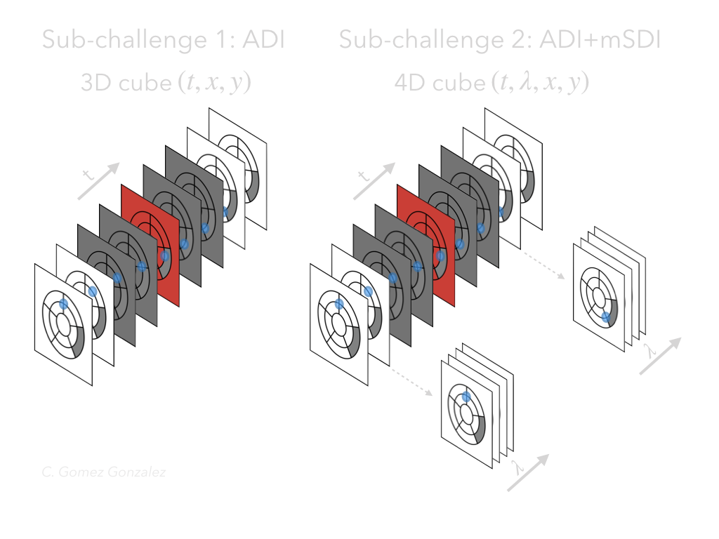
Multi-spectral imaging is usually combined with ADI in modern instruments. In this case, the datasets are composed of a 4d cube of images (see Fig. 2), a vector of parallactic angles, a vector of wavelenghts and a PSF (this is detailed in the datasets section of this website).
 |
|---|
| Figure 2. Dimensionality of the cubes used in this challenge, depending on the observing technique: the left panel shows a single ADI data cube and the right panel shows an ADI + multi-channel SDI data cube. |
Note on RDI: Although Referential Differential Imaging (RDI) does not constitute a separate sub-challenge, we welcome submissions that make use of reference datasets or libraries (whether it is the cubes provided within the challenge or external ones). We only require the participant to make clear if RDI is used instead of pure ADI or ADI+mSDI post-processing (this is explained on the “metrics” sub-section on the top navigation bar).
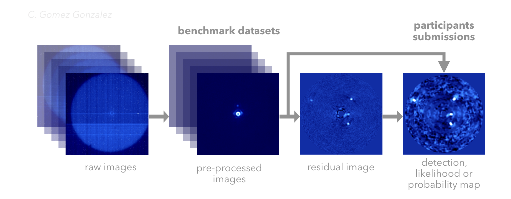
In Fig. 3 we show an schematic representation of a HCI blob/planet detection pipeline. In the context of this data challenge, we will not use datasets with known (real) companions. Instead, we will inject synthetic planets or companions in order to measure the detection capability of different algorithms. Each challenge cube contains from none to five synthetic point-sources, injected using a standard process without accounting for smearing or variable photometry). For spectrally dispersed data we will use three template spectra when injecting the fake companions.
 |
|---|
| Figure 3. Schematic representation of the high-contrast imaging data processing pipeline, for the case of a LBTI/LMIRCam HR8799 data cube. Notice how from a data cube (or image sequence) we obtain one view of the star’s vicinity and an associated detection map where we could detect potential point-like sources. |