Codalab competition: The challenge is hosted on Codalab, please follow this link. In order to participate, you must first register as a Codalab user.
WARNING: The backend implemented in CodaLab contains an error that we cannot modify during the competition. Please do not consider the F1-score shown on the CodaLab leaderboard. Proper analysis of the results will be done offline at the end of the competition.
This challenge is focusing on the task of exoplanet direct detection. In order to measure the detection capability of different algorithms, we will rely on the injection of fake companions and the computation of several relevant metrics, such as the true positive rate or the number of false positives.
On the table below, you can find a summary of the metrics used for each stage:
| Sub-challenge 1: ADI | Sub-challenge 2: ADI+mSDI | |
|---|---|---|
| Stage | Metric | Metric |
| 1 | F1, TPR and FDR | F1, TPR and FDR |
| 2 | ROC space | ROC space |
Stage 1: By thresholding each detection map (using the provided value_threshold for claiming a detection) and counting the true and false positives, we define several metrics:
- the true positive rate (TPR) also known as sensitivity or recall:
TPR = TPs / Ninj, - the false discovery/detection rate (FDR):
FDR = FPs / Ndet, - the precision or positive predictive value (PPV):
PPV = TPs / Ndet, - the F1-score or harmonic mean of TPR and the precision:
F1 = 2 * PPV * TPR / (PPV + TPR).
where TPs is the number of true positives/detections, FPs is the total number of false positives or Type I error, Ndet is the total number of detections (TPs + FPs) and Ninj is the total number of injections (accros all the datasets of a given sub-challenge). The TPs, FPs and Ndet are counted for a given participant/algorithm over all the datasets of a given sub-challenge. This blob counting procedure is implemented in the Vortex Image Processing package, specifically in the vip_hci.metrics.compute_binary_map() function (https://github.com/vortex-exoplanet/VIP/blob/master/vip_hci/metrics/roc.py). Read below about the Challenge starting kit Notebook, which contains detailed explanations about the blob counting procedure.
Two scoreboards will be computed, one for the sub-challenge on ADI data (3D cubes) and one for the sub-challenge on ADI+mSDI cubes (4D cubes). The F1-score serves well our goal of assessing the performance of detection algorithms as binary classifiers, therefore we will use it to rank the entries on each scoreboard.
The contrast (brightness) value for injecting each synthetic companion will be estimated wrt a baseline algorithm. First, the S/N of a population of injected companions will be measured on residual final frames (processed with the baseline algorithm). Then, the interval of fluxes as a function of the separation from the star will be defined by checking which contrast corresponds to S/Ns in given interval (e.g. 1 to 4). This procedure is implemented here.
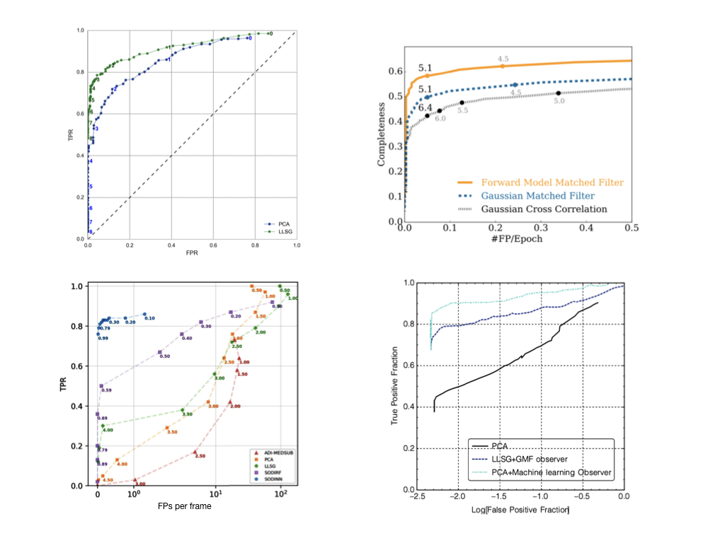
Stage 2: The community is converging on the usage of receiver operating characteristic (ROC) curves for the performance assessment of high-contrast imaging post-processing algorithms (see Jensen Clem et al. 2017). In Fig. 3 is displayed a compilation of some ROC curves from the high-contrast imaging literature.
 |
|---|
| Figure 3. ROC curves in the high-contrast imaging literature. Top-left from Gomez Gonzalez et al. 2016, top-right from Ruffio et al. 2017, bottom-left from Gomez Gonzalez et al. 2018 and bottom-right from Pueyo 2018. |
In this stage, we will focus on the computation of ROC curves for comparing the trade-off of TPR and number of FPs for different algorithms as a function of the detection threshold. The ROC curve computation boils down to repeating the above procedure of injecting companions in the empty challenge datasets, computing detection maps, thresholding them and counting sources, ie. the detection state and the number of false positives for different detection criteria. This expensive procedure will be performed locally using the source code of the algorithm submitted by each participant.
Codalab
Instead of re-inventing the wheel (designing a service to host the data challenge submissions ingestion program), we chose to run this challenge on Codalab, a framework for accelerating reproducible computational research. The participants will enter the competition by creating their own account on Codalab and following the link to the challenge.
Codalab displays four tabs: Learns the details, phases, participate and results. Please note our two sub-challenges correspond to phases in Codalab. Both sub-challenges (phases in Codalab’s jargon) will be open until the end of the competition. Each sub-challenge will have a separate scoreboard, which will be updated automatically with every new submission to the Codalab interface. The challenge interface will offer the option to include a short description of the algorithm you used for a each submission, please don’t forget to fill in this information (specially if the algorithm uses RDI or some sort of black magic). Participants may submit as many times as they want. The scoring routines that compute the metrics can be found on the Data Challenge Extras repository.